While quarantined in NYC I’ve finally worked through the classic text on reinforcement learning. This is the first of a 4 part summary of the text intended for those interested in learning RL who are not interested in staying in their apartment for three months to learn it .

overview

motivation

Despite their neuro-inspired-namesakes, many modern deep learning algorithms can feel rather “non-biological”. Consider how living things learn. To teach my nephew the difference between cats and dogs, I do not show him thousands of cats and dogs until the (non-artificial) neural networks in his brain can distinguish them. This sort of training is well-suited to machines but not minds.

Moreover, much of what he learns is via direct interaction with the world. He knows what he likes and doesn’t like, and through trial and error he maximizes the good stuff and minimizes the bad stuff. Although this isn’t the only way animals learn (despite what some psychologists used to think), it is a powerful approach to navigating the world.

Reinforcement learning uses this idea to power algorithms that are sometimes superhuman. Sutton & Barto is the classic introductory text on the subject. This is part 1/3 of my summary of the text. We will introduce the general reinforcement learning problem (along with necessary terminology and notation), and then describe dynamic programming and Monte Carlo reinforcement learning algorithms.

setup

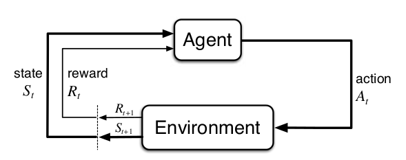
In reinforcement learning an agent collects reward by acting in an environment. The actions of the agent, together with the dynamics of the environment, determine $(1)$ how much reward the agent gets and $(2)$ how the state of the world changes. The agent selects actions using a policy, which defines how likely all actions are in a given state. The goals is to find a policy that gets us as much reward as possible.

At time $t$ the state of the environment is $S_t \in \mathcal{S}$ and an agent can take an action $A_t \in \mathcal{A}(s)$. Notice that the actions available to the agent depend on the state $s$. The environment then emits a reward $R_{t+1} \in \mathbb{R}$ and a subsequent state, $S_{t+1}$. The reward is just a scalar! From this sparse information the agent must figure out how to maximize reward. This should seem somewhat surprising and magical.

The interactions between an agent, its actions, and the environment can be usefully modelled as a Markov Decision Process (MDP). In Markov systems the current state of the world determines (potentially stochastically) the next state of the world. If you know the current state, there is no dependency on past states. In other words, the future is independent of the past given the present:¹

Given a state $s$ and action $a$, the probability of moving to a new state $s’$ with reward $r$ is given by the following. Note that the function $p$ maps four arguments (the current state, the next state, the action, and the reward) to a probability between $0$ and $1$, i.e. $p : \mathcal{S} \times \mathcal{S} \times \mathcal{A} \times \mathcal{R} \rightarrow [0,1]$.

The function $p(s’,r \mid s,a)$ describes the dynamics of the environment. In model-based reinforcement learning we know (or learn) these dynamics, whereas in model-free reinforcement learning they are not used.

returns

Our policy should not only encourage the acquisition of immediate reward, but also future reward. We therefore want to maximize returns, which are a function of reward sequences. For example:

This is an undiscounted return because it equally weights all rewards. It is common to exponentially discount future rewards using a discount factor $\gamma$. When discounting, future rewards matter less than immediate rewards (interestingly, people and animals appear to follow this principle):

Note that we can define returns recursively just by rearranging some terms. This simplifies the equation, and establishes a recursive relationship that is critical for many ideas in reinforcement learning:

value functions

How can we maximize our return? Recall that an agent selects behaviors according to some policy, which is a function with learnable parameters. A first thought might be to optimize the parameters of the policy with respect to overall return (we’ll get to these policy gradient methods in part 3). An alternative approach is to learn how good different states are. We can then maximize returns by selecting actions that move us to the best states.

A value function describes how good different states are. Specifically, it tells us how much return we expect in a given state. Because the return depends on the actions we select, the value function will also depend on the policy $\pi$, hence the subscript in the following equation:

Plugging in the recursive relationship we established above we have:

To take expectations over the random variables $R_{t+1}$ and $G_{t+1}$, we have to sum across all possible values for these variables, weighted by their correspodning probability.

Let’s unpack this equation. How valuable is a state? It depends on $(1)$ what action you take, $(2)$ the reward you get from that action, and $(3)$ the value of the state you end up in. $(1)$ means we must average over possible actions, weighted by their probabilities (the first summation), and $(2,3)$ mean we must average over possible states and rewards that could result from that action, again weighted by their probabilities (the second summation). Therefore, $\sum_a \pi (a \mid s) \sum_{s’, r} p(s’,r \mid s,a) \dots$ averages over all possible combinations of $a$, $s’$, and $r$.

Finally, we will use the fact that the expected return for the subsequent state is the value of the subsequent state. This allows us to replace the bracketed term on the right as follows (notice that we’re using that recursive trick again to simplify notation!):

We have now arrived at the Bellman equation, which recursively relates $v_\pi$ to itself. It states that the value of a state is the reward expected immediately (averaging across all actions), plus the discounted value of the subsequent states (averaging across all subsequent states for each action).

$v_\pi(s)$ is a state-value function because it reports the value of specific states. We will also consider action-value functions, which report the value of state-action pairs (answering the question “How good is it to take action $a$ in state $s$?”):

An optimal policy yields the highest possible return. The optimal state-value and action-value functions are denoted $v_{* }$ and $q_{* }$, respectively, and reflect the value of each state (or each state-action pair) under the assumption that the agent follows the optimal policy thereafter. They can be recursively defined using the Bellman optimality equations:

In the previous Bellman equations we took the expectation over actions; for the Bellman optimality equations we take the max instead. This means that an optimal policy will always select actions that lead to the highest value subsequent state. Keep in mind that the value of a state is a function of all future rewards, so sometimes the optimal policy sacrifices immediate reward for larger reward in the future!

dynamic programming

bootstrapping the value function

We usually don’t have complete access to the state of the world and its dynamics². When we do, model-based algorithms such as dynamic programming³ can be used to iteratively converge on optimal policies. Keep in mind that the term dynamic programming refers to a broader class of algorithms that extend beyond reinforcement learning. Generally, they are algorithms in which a problem is decomposed into solvable sub-problems. If the same sub-problem is repeatedly encountered we can store and re-use its solution.

Recall that the Bellman equations define a recursive relationship for value functions. We can therefore bootstrap, using our (initially inaccurate) estimate of the value of subsequent states to figure out the value of the current state. Notice that we are using the solution to a previous problem (the value of $S_{t+1}$, which the agent will likely have seen before) to solve our current problem (the value of $S_{t}$). With this logic we can turn the Bellman equations into recursive update rules that can be iteratively applied to converge on accurate value functions. These value functions can then be used to construct optimal policies.

Before we can improve our policy, we need a way to measure how good our current policy is. This is called policy evaluation, or prediction⁴. This is the process of determining the correct value function for a particular policy. We are not improving our policy yet; rather, we are trying to figure out how good each state is under the current policy.

In dynamic programming we do this by turning the Bellman equation for $v_\pi$ into an update rule. Now we are iteratively improving our value function, and $v_k$ refers to the value function at iteration $k$:

In other words, $v_{\pi}$ is estimated as the reward we expect immediately plus the discounted value of the next state. Because both the policy and environment are (potentially) stochastic, we need to average over all possible $a$, $s’$, and $r$. Notice that this approach is biased (it will not be correct on average); we are using an (initially) inaccurate estimate of subsequent states to update the value of the current state. Nonetheless, it can be shown that repeatedly applying this update (by looping over all states) will cause convergence to the true value function. Awesome.

Now that we have an accurate value function we can update our policy. All we have to do is act greedily with respect to it. This means selecting actions that lead to the highest value states. For example, if our policy says go left, but our value function says going right will lead to greater return, we update our policy accordingly.

generalized policy iteration

So far so good - but wait! Our value function was defined with respect to $\pi_k$, but now we’ve updated the policy to $\pi_{k+1}$, which means our value function is no longer accurate . We therefore need to go back and update our value function again.

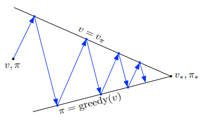
By repeating the process of updating our value function for a given policy (policy evaluation) and then updating our policy based on the new value function (policy improvement), we can converge on an optimal policy, $v_*$. This framework, which is common to many reinforcement learning algorithms, is know as generalized policy iteration.

In the following visualization, the upward arrows represent policy evaluation, wherein our value function $v$ gets closer and closer to the true value function for the current policy, $v_\pi$. The downward arrows represent our policy improvement step, wherein we act greedily with respect to our updated value function. By repeating this process we converge towards the optimal policy, $\pi_* $ and its associated value function $v_* $.

value iteration

In the dynamic programming algorithm we just described, we must iteratively improve our value function after every policy update. How many times should we improve the value function for a given policy? Do we need to wait until it’s nearly perfect? It turns out that even an imperfect but improved value function can help us find a better policy. In the extreme, we can update our value function just once for a given policy, and always act greedily with respect to that value function. This is called value iteration.

Let’s see what this looks like algorithmically. To update our value function we apply our previous dynamic programming update rule just once for all states:

Because the policy is always greedy with respect to the current value function, $\pi(s \mid a)$ is zero for all but the best action, which has probability $1$. Therefore, rather than taking the expectation over actions we can simply take the max . This gives us a nice, compact update rule (which should look suspiciously similar to the Bellman optimality equation):

Notice that the policy has disappeared from our equation. With this sleight of hand we are now working totally in “value function” space. Only after our value function has converged do we set the policy to be greedy with respect to it.

limitations of dynamic programming

Dynamic programming requires that we know how the world works. This is a lot to ask. To take expectations over actions and the states/rewards that result from those actions we need a model that tells us how the world reacts to what we do. Concretely, this means we need $p(s’,r|s,a)$ to be given⁵.

Furthermore, we must loop over all states in the environment. This is feasible when the number of states is small (e.g. possible board configurations in tic-tac-toe), but not when the number of states is large (e.g. possible board configurations in chess). We therefore need methods that work in the real world, which is big, scary, and full of states .

monte carlo methods

figure it out by sampling!

How can we estimate the value function when we don’t know the dynamics of the environment? Here’s a simple but powerful idea for model-free learning. Recall that the value function is the expected return for a state (or state-action pair):

Monte Carlo methods⁶ estimate value functions by simply averaging sample returns. For example, $v(S_t)$ would be the average return we get following visits to state $S_t$. The estimates may be noisy (high variance) but will be correct on average (zero bias), and with enough samples they will be quite accurate. We can then find good policies by acting greedily with respect to these value functions.

prediction

Let’s make this concrete by describing a Monte Carlo prediction algorithm (remember, “prediction” means figuring out the value of states under our current policy). First we define an episode (or rollout, or trajectory) to be a series of states, actions, and rewards that ends in a terminal state at time $T$. Think of this as a single ‘experience’ the agent can learn from:

In the following algorithm we will generate episodes by following our policy. When we reach a state for the first time during an episode, we update its value to be the average return for that state across all episodes.

Annoyingly, we need full trajectories before updates can be performed (because returns are functions of all future rewards). We therefore wait until the end of an episode to update values for visited states. To do this we loop backwards in time, performing updates only for first visits to states in the trajectory (there are also every visit methods, which update with every visit to a state in the trajectory):

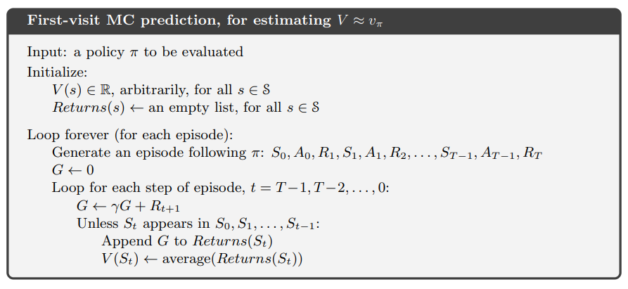
Notice that setting $G \leftarrow \gamma G + R_{t+1}$ when looping backwards from $T-1 \rightarrow 0$ causes $G_t$ to equal $R_{t+1} + \gamma R_{t+1} \gamma^2 R_{t+2} \dots \gamma^{T-1} R_{T}$, as desired.

encouraging exploration

In dynamic programming we looped over all states to update the value function. In Monte Carlo we generate data by letting our agent behave in the environment. This is nice because updates will focus on states that are actually relevant to our policy. However, the agent may not explore the environment enough, which means very valuable states may never be discovered.

We’ve hit upon a fundamental problem in reinforcement learning. The goal is to maximize returns. To do this, we take actions we believe to be the best. However, discovering new, better actions requires sometimes testing actions we are unsure of. The tension between exploitation of what we know to be good and exploration to discover better actions is fundamental. A typical example is the decision to dine at your favorite restaurant (exploit) or try a new restaurant (explore)⁷.

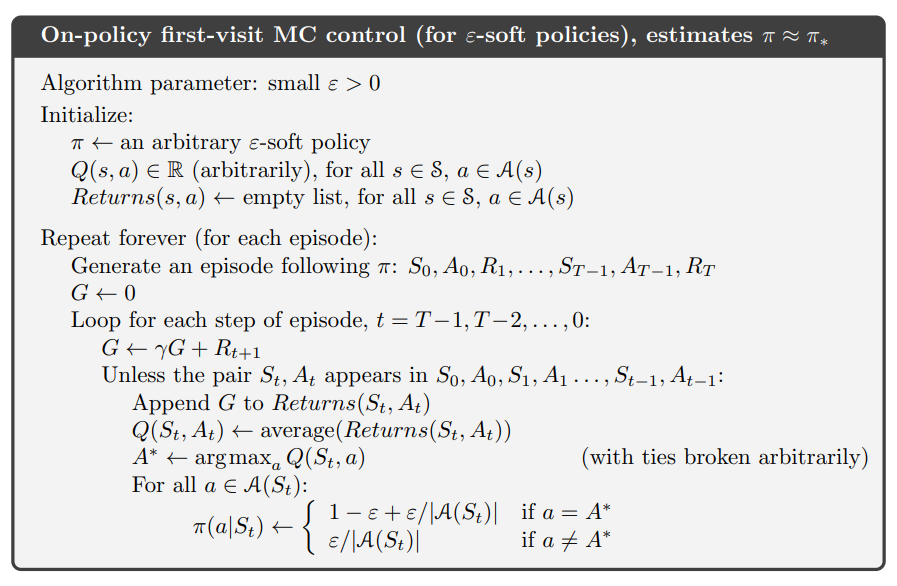
How can we ensure our agent tries potentially valuable actions that are not favored by the current policy? One approach is to adopt stochastic policies that usually pick the “best” action, but sometimes pick actions at random. So-called $\epsilon$-greedy policies select the estimated best action with probability $(1-\epsilon)$ and random actions with probability $\epsilon$. There are more intelligent ways of exploring the world, but this simple trick proves very useful in many circumstances.

control

Now that we have a Monte Carlo method for learning value functions we are ready to find good polices. When the environment dynamics $p(s’,r \mid s,a)$ are known, moving from the state-value function $v_\pi$ to an improved policy is trivial; we simply select actions that lead to more valuable states. How can we select good actions when we don’t know which actions lead to which states, i.e. when $p(s’,r \mid s,a)$ is not known?

This is where the action-value function $q_\pi(s,a)$ comes in. If $q_\pi(s,a)$ is accurate, we don’t need to know how our state evolves as a function of our actions. All we need to do is pick the action that maximizes $q_\pi(s,a)$:

In the following algorithm we learn $q_\pi(s,a)$ using the first-visit Monte Carlo approach described above. Furthermore, it uses $\epsilon$-greedy action selection to encourage exploration:

off-policy prediction

A very powerful way to ensure the state space is adequately explored is to have separate behavior and target policies. The behavior policy guides behavior during data acquisition whereas the target policy is actually being evaluated. Using an exploration-heavy behavior policy can encourage exploration of states that may be seldom visited under the target policy.

There’s an important catch: if we average returns from trajectories sampled under the behavior policy, we will estimate expected returns under the behavior policy, whereas we want to evaluate the target policy . To address this, we can weight each return by its likelihood under target policy relative to the behavior policy. This weight is call an importance sampling ratio and is defined as:

Here $b$ is the behavior policy and $\rho_{t:T-1}$ is the weight associated with the trajectory occurring between times $t$ and $T-1$. By weighting the returns with $\rho_{t:T-1}$, the expected value of our estimate becomes the true value under the target policy (i.e. there is zero bias).

Ordinary importance sampling estimates the value of a state $s$ by averaging the returns from all visits to $s$, each weighted by $\rho_{t:T-1}$. In the following equation, $\mathcal{T}(s)$ is the set of all times state $s$ was visited and $T(s)$ is the time at which the episode containing time $t$ terminated. $V(s)$ is our estimate of the true value function, $v_\pi$.

This approach has zero bias (it will converge to the desired expected value) but has very high variance. For example, if $\rho_{t:T-1}$ is large it can drastically overweight some returns. An alternative approach called weighted importance sampling uses a weighted average for trajectories. A weighted average has weights that sum to 1. To accomplish this we divide by the sum of all $\rho_{t:T-1}$. This approach has lower variance but higher bias.

Off-policy learning can be useful for exploration, but there is another advantage. Imagine you are optimizing a policy for a self-driving car, and you have access to data from old self-driving cars. Rather than testing your policy by letting your car drive around (a time-consuming, expensive, and potentially dangerous exercise for an untested policy), you can evaluate your policy according to the experience of the old cars. This gives you instant access to a wealth of training data.

up next

The methods we just learned work well for tabular state spaces - those in which there are (a reasonably small number of) discrete states. Most interesting problems are much more complex! In part 2 we will learn to estimate value functions using function approximation, which will allow us to handle large and/or continuous state spaces.

acknowledgements

Thank you Chris Rodgers for providing very helpful feedback on this post. If you were disappointed that I didn’t sufficiently unpack the equations, know that your disappointment would have been greater had I not incorporated Chris’s suggestions.