In part 1 we discussed dynamic programming and Monte Carlo reinforcement learning algorithms. These appear to be qualitatively different approaches; whereas dynamic programming is model-based and relies on bootstrapping, Monte Carlo is model-free and relies on sampling environment interactions. However, these approaches can be thought of as two extremes on a continuum defined by the degree of bootstrapping vs. sampling. Temporal difference is a model-free algorithm that splits the difference between dynamic programming and Monte Carlo approaches by using both bootstrapping and sampling to learn online.

temporal difference learning

combining bootstrapping and sampling

Let’s step back and consider the differences between dynamic programming and Monte Carlo. In Monte Carlo we estimate $v_\pi$ by sampling and averaging returns. In dynamic programming, we bootstrap, using the estimated value of subsequent states to figure out the value of the current state. Temporal difference (TD) learning is a model-free approach that combines sampling and bootstrapping. It is an important idea both in reinforcement learning and neuroscience.

Recall that in Monte Carlo we compute returns from full trajectories of experience:

This means we have to wait until the experience is over to compute the return¹ . In TD learning we estimate returns after observing only $R_{t+1}$, relying on the fact that returns can be expressed recursively:

Finally, in our estimated return (which we will call a target for reasons that will soon become clear), we will replace $G_{t+1}$ with our estimate of the value of the next state, $V(S_{t+1})$. This is reasonable because $v_\pi(S_{t+1}) = \mathbb{E}[G_{t+1} \mid S_{t+1}]$ (see part 1 of this series for details).

Notice the trick here. In Monte Carlo we had to sample entire returns (not fun) to estimate the value of a state. Now we’re just sampling a single reward $R_{t+1}$, then we estimate the rest of the return by bootstrapping with our previous estimate of the value for the subsequent state. So we are sampling (a la Monte Carlo) and bootstrapping (a la dynamic programming).

Okay! In Monte Carlo we estimated a state’s value as the average return for that state. Similarly, we can compute the average target for each state by storing all targets for all states, then summing and dividing by the number of targets for each update. However, st oring all of the targets for each visit to each state is not ideal. Fortunately, the following incremental update rule is mathematically equivalent to averaging, but it only requires storing the number of times each state is visited, $N(s)$:

This equation says that the new average target is just the old average, plus the difference between the target (in blue) and the the old average multiplied by a scaling factor.

There is some intuitive appeal here. At every step, the target is compared with the current value estimate. When the target is higher than the expected return (i.e. when we get more reward than we expect), we increase the value function for this state. We we get less than we expect, we decrease the value function. In other words, we move our estimate a little bit towards the target 😁.

The difference between the target and the return is called the TD error, $\delta_t$. It tells us how “surprised” we should be be the estimated return we just observed.

Let’s make one last adjustment to our update rule. When we average estimated returns, we assign equal weight to returns collected at all times. This makes sense for stationary environments - those with unchanging dynamics. But many environments change over time. Consider a chess opponent who learns your style of play over the course of the game. Her strategy (which is part of the environment) will change, and your value function should change accordingly.

For these reasons it often makes sense to weight recent experiences more heavily when averaging. By replacing $\frac{1}{N(S_t)}$ with a learning rate $\alpha \in [0,1]$, we have an exponentially weighted average that ‘forgets’ old episodes over time:

Using this update rule we can create algorithms for prediction (figuring out how good different states are under the current policy; see part 1). Now let’s consider how we can use TD learning to find good policies.

Recall that state-value functions $v_\pi(s)$ aren’t terribly useful if we don’t know the environment dynamics $p(s’,r \mid s,a)$. Knowing the values of different states doesn’t help if we don’t know which actions lead to which states! Therefore, as we did with Monte Carlo control, we will learn action-value functions $q_\pi(s,a)$ instead of state-value functions, and select actions that maximize $q_\pi(s,a)$.

backup diagrams

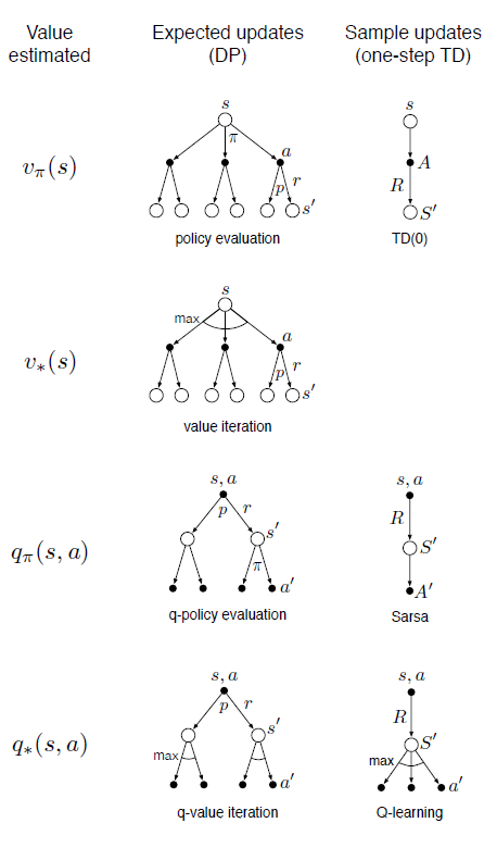
The following algorithms can be nicely illustrated using backup diagrams like these:

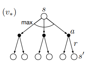
In backup diagrams, states are represented by open circles and actions by black dots. Transitions from states (circles) to actions (dots) are governed by the policy $\pi(a \mid s)$. Transitions from actions (dots) to subsequent states (circles) are governed by the environment dynamics $p(s’,r \mid s,a)$. Each transition from an action to a subsequent state is associated with a certain reward $r$.

Notice that there are several actions available at each state, and each of these has a probability determined by the policy. Similarly, because environments will often be stochastic, each state-action pair $(s,a)$ can result in several possible subsequent state-reward pairs $(s’,r)$

Oftentimes we want to take expectations over actions or subsequent states, e.g. when computing value functions in dynamic programming (see part 1). To do this we take probability-weighted averages across the arrows emanating from a particular state or action node. In other cases we want to pick the best possible action, e.g. in value iteration (see part 1). To do this we take the max rather than the expectation across actions, which is denoted by arc in the diagram above.

SARSA

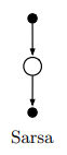
We can learn action-value functions using an update rule analogous to the state-value update described above. Given a State, we select an Action, observe the Reward and subsequent State, and then select the next Action according to the current policy. The target is the reward we get immediately, plus the discounted value of the next state-action pair, $\color{blue}{R_{t+1} + \gamma Q(S_{t+1}, A_{t+1})}$. Using this target, the update rule for SARSA is:

Note that this is an on-policy method because were are always selecting actions according to the current policy.

Q-learning

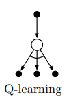
SARSA learns the action-value function associated with a given policy. The policy can then be improved by acting greedily with respect $Q(s,a)$. Q-learning is an off-policy algorithm that directly approximates $q_{* }(s,a)$, which is the action-value function associated with the optimal policy $\pi_{* }$. To do this, we take the best action when bootstrapping, as opposed to the action chosen by our current policy:

Note that this is an off-policy algorithm because actions aren’t selected according to the current policy.

expected SARSA

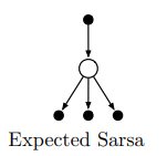
Recall that policies define probability distributions over actions. In SARSA, $A_{t+1}$ is therefore a random variable distributed according to our policy. For stochastic policies (such as $\epsilon$-greedy), this introduces variance in our action-value estimates that can be mitigated by taking expectations over actions. This is called expected SARSA.

Here we don’t select the second action, but instead average over actions we could take weighted by their probabilities. Because the expectation is with respect to the policy-determined distribution over actions, expected SARSA is considered on-policy (although you could in principle take expectations over actions according to a different policy, in which case it would be off-policy ).

$\lambda$ return

splitting the sampling-bootstrap difference

Quick recap: Dynamic programming relies on bootstrapping and is low variance but high bias. Monte Carlo relies on sampling and is high variance but low bias. Temporal difference learning combines sampling and bootstrapping and therefore splits the difference in the bias-variance tradeoff.

Wouldn’t it be nice to dial in the precise contributions of sampling and bootstrapping? Then we could strike a balance between bias and variance that suits our problem. The following methods accomplish this by varying the extent to which we sample vs. bootstrap during our value function updates.

n-step bootstrapping

In TD learning we estimate returns by taking one step in the environment, observing $R_{t+1}$, and then bootstrapping. But nothing is stopping us from taking $n$ steps before bootstrapping. Notice that when $n \rightarrow \infty$ we have Monte Carlo learning again!

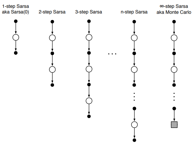
The $n$ step return and its associated update rule (for state-value functions) are:

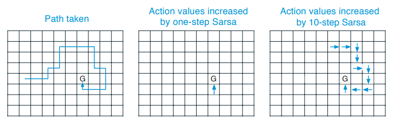
Intuitively, taking larger $n$ allows us to see further back when assigning credit/blame to states and actions that led to reward. For example, upon reaching a reward state when $n=1$ we only updated the value of the states/actions that caused reward, but the actions that led to the actions that caused reward are not updated. With $n=10$, however, we can assign credit to several states in the sequence that resulted in reward:

$\lambda$ return

$n$-step returns ($G_{t:t+n}$) allow us to control the extent to which we rely on sampling (big $n$) vs. bootstrapping (small $n$). Rather than picking a single $n$, we can take take an exponentially weighted average of $n$-step returns for all $n$. For $\lambda \in [0,1]$ we have:

The $(1-\lambda)$ term ensures the weights sum to 1. Note that for $\lambda=0$ this reduces to a one step return, whereas for $\lambda=1$ it is a monte carlo return.

For continuous settings we can’t compute $n$-step returns for arbitrarily large $n$. We can therefore approximate $G_t^\lambda$ by taking the first $k$ returns. The trick is to “pretend” that all of the returns after time $k$, $G_{t:t+k+\delta}$ for $\delta \in \mathbb{N}$, are the same as the last return, $G_{t:t+k}$. By setting all $G_{t:t+k+\delta} =G_{t:t+k}$ we effectively give all the residual weight in our exponentially weighted return to the $k^\text{th}$ time step:

offline $\lambda$ return algorithm

The offline $\lambda$ return algorithm performs weight updates after each episode according to the $\lambda$ return at each time point using semi-gradient ascent as follows:

online $\lambda$ return algorithm

We can perform truncated $\lambda$ return updates online, but this requires a trick. If we are interested in $5$-step $\lambda$ returns, but we are only at $t=2$, we start by computing the $2$ -step return. Then when $t=3$, we go back and update our previous weight updates using the most recently available returns, and so on.

forward vs. backward views

Quick recap of TD learning: every time we encounter a state, we update it’s value in the direction of immediate rewards, and to a lesser extent distant rewards. We continue moving state by state, associating rewards with states based on their temporal proximity.

If a reward occurs soon after a state, we associate the reward with the state. By the same token, if a state occur soon before a reward, we should make the same association. This backward view is appealing because it opens the door to efficient, online algorithms for value function updates.

In the backward view we need to keep track of how recently we visited each state, because we want to associate rewards more strongly with recently visited states. Just as rewards are discounted exponentially as time passes, our recency metric will fade exponentially. This recency metric is called an eligibility trace, which we will encode in a vector $\mathbf{z}$ that has one element per state. Each element tells us how recently that state was visited.

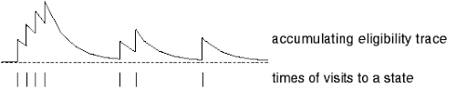
If $\mathbf{x}(s)$ is a one-hot vector representation of the state, then when we visit state $s$ we will update the eligibility trace according to:

This says that when we visit a state (when $\mathbf{x}(s)_i=1$) we “bump up” its value in the eligibility trace. Otherwise (when $\mathbf{x}(s)_i=0$), the trace decays exponentially. For each state this causes decay patterns like this:

TD($\lambda$)

TD($\lambda$) approximates the offline $\lambda$-return using an efficient backward view algorithm. We first need to generalize eligibility traces to value function approximation (see part 2). Recall that if we have a value function approximation $\hat{v}(s, \mathbf{w})$ parameterized by weights $\mathbf{w}$, the general formulation for the weight updates is:

where $\alpha$ is the learning rate and $\delta_t$ is the TD error - the difference between the target and our current value estimate. $\delta_t$ tells us how much we should be surprised by what is happening now. We will use a new eligibility trace update rule:

This more general eligibility trace no longer strictly reflects the recency of states. At each time point, $\nabla \hat{v}(S_t, \mathbf{w}_{t})$ tells us how we would change each element in $\mathbf{w}$ to increase the value estimate of $S_t$. This means $\mathbf{z}$ is now like a smeared-out version of the gradient. It reflects how eligible each element in $\mathbf{w}$ is for tweaking when something good or bad happens.

We will now modify our weight update by using this smeared-out version of the gradient intead of the original gradient:

Let’s consider how this update rule works. When things go better than expected, $\delta_t$ will be high. We then nudge $\mathbf{w}$ in the direction that increases the value of recent states, because $\mathbf{z}$ contains the gradients for past states weighted by their recency². Whereas our original update rule only cared about the current gradient, our $\mathbf{z}$-based update “see backwards” into the past a bit. Nice.

true TD($\lambda$) and dutch traces

TD($\lambda$) only approximates the offline $\lambda$-return. However, by tweaking the eligibility trace and weight update formulas, we can achieve a backward view algorithm that is equivalent to the online $\lambda$-return. The new dutch trace and associated weight update are:

A proof for the equivalence of the forward and backward views using dutch traces is provided in the text for the case of Monte Carlo control without discounting (section 12.6).

the big picture

breadth vs. depth

The methods we’ve applied so far vary in breadth and depth. Methods that bootstrap can be thought of as “shallow” in that they only step a little into the future (TD learning) or not at all (dynamic programming) before bootstrapping on the value function estimate. Monte Carlo, on the other hand, is “deep” in that it samples until the end of trajectories.

Furthermore, methods that take expectations over actions (dynamic programming) are “wide”, whereas methods that take specific actions (TD learning and Monte Carlo) and “narrow” because they rely on sampling rather than averaging over actions.

Methods exist in between these extremes and can be thought of as living in a space characterized by two axes. These axes represent the extent to which a method relies on sampling vs. expectations (narrow vs. wide), and bootstrapping vs. sampling (shallow vs. deep):

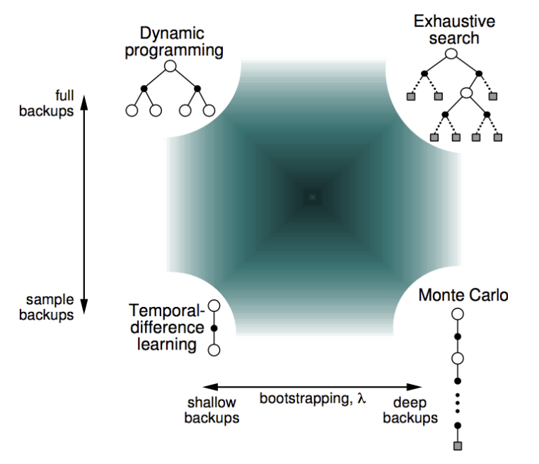
Where you should live in this space depends on the problem you are solving! Increasing your reliance on bootstrapping reduces variance but increases bias. Taking expectations over actions reduces bias but increases computational complexity.

value function updates

We’ve learned several methods for updating our value function so far. Now is a good time to step back and taxonomize³ them a bit.

The updates we’ve considered differ in whether they (1) update the state vs. action value function, (2) approximate the value function under the optimal ($v_*(s)$) vs. the current policy ($v_\pi(s)$), and (3) rely on sampled vs. expected updates. The different combinations of these three binary dimensions yield the following family of value function updates:

up next

In parts 1-3 we learned how to learn value functions. We then found good policies by choosing actions that maximized these value functions. Notice, however, that these methods generally require discrete action spaces (the agent can only take one of several distinct actions). Part 4 covers policy gradient methods, which find policies directly by optimizing their parameters with respect to a loss function. This will open the door to powerful techniques for continuous control.